Introduction
Autogasuptake is a convinient tool for automating the calculation and visualization of gas uptake from a raw csv file that contains the cylinder volume and the pressure of the gas in the experimental system.
Requirements
You will need below packages to run Autogasuptake. But don't worry, you can install them all with pip or pip3. Personally, I'm highly recommend you to use Anaconda as your Python distribution.
pandasmatplotlibnumpyscipyscikit-learnseabornpyfiglettabulate
Features
- Can polish the raw data file
- z value calculation based on Peng-Robinson & Redlich-Kwong EOS models
- Can calculate the gas uptake based on the z value
- Supply various user options
- Can decorate the graph with research figure style
- Can export the graph as a png, pdf, or svg file
How to Install
It is easy to install Autogasuptake. Just use pip or pip3 to install it.
pip install autogasuptakeor
pip3 install autogasuptakeHow to Use
(1) Graph plotting
After installing Autogasuptake, you can execute it right in the terminal. But before you use it, you need to prepare csv files from your experimental data (mainly came from the LabVIEW program). Note that LabVIEW program exports the data in a csv file with space as the delimiter (but it's ok if you use comma (',') as delimiter. The program automatically recognizes this and proceeds with data processing normally). It looks like this:
570.000000 406.754852
569.799988 406.006744
569.799988 404.104126
569.799988 401.781738
The first column is the pressure (psi) of your system, and the second column is the volumn (mL) of the cylinder. Make sure to remember the location where you save these raw csv files.
Then, deploy Autogasuptake in your terminal.
autogasuptakeThe program initiates, and firstly asks you to make the settings.txt file if you don't have one.
ERROR There is no `settings.txt` file in the current directory. I will make a new `settings.txt` file for you.
INFO The `settings.txt` file has been created. Please edit the file and run the program again.
If you have already have your own settings.txt file, you won't see this message.
The exported settings.txt file looks like this:
###################################
############ SETTINGS.TXT #############
###################################
# NOTE: This file should be located in the directory where you are executing the program. This can be done by typing `pwd` in the terminal. Check your current location.
# NOTE: You can mark `#` in front of the lines you don't want to use.
# NOTE: This file should be named as `settings.txt`. If isn't, the program cannot load the settings.

###########################################################
# Target directory where the raw data files are located.
directory = ./

# Data collection frequency (in ms); the value when you set in the LabVIEW program.
frequency = 300000

# Experimental temperature (in K)
temperature = 276.3

# Critical temperature of your interested gas (in K)
tc = 209.5389

# Critical pressure of your interested gas (in bar)
pc = 55.034

# Acentric factor of your interested gas
omega = 0

# Time unit (h, m, or s)
tunit = m

# Whether to decorate the graph with research figure style (options: y, n)
graph-decorate = y

# Plot type (options: line, scatter)
plot-type = scatter

# Whether to include the title in the graph (options: y, n)
include-title = n

# Output file type (options: png, pdf, svg)
output-file-type = png

# Equation of state model (options: rk, pr)
eos = pr

# Water mass you used in the experiment (in g)
water-mass = 50

# Type of the clathrate (options: sI, sII, sH, SCS-I, TS–I, HS-I, and none)
clathrate-type = sII- Basically, you should choose your interested gas and find its critical temperture, critical pressure, and acentric factor. And carefully modify
settings.txtfile according to your found values. Note that the demosettings.txtfile is written for the calculation of gas uptake of molecules. - After then, you can choose whether to decorate the graph with research figure style, whether to include the title in the graph, and the output file type. Especially, if you choose
yfor the graph decoration, the program will change the font-style, font-size, and line-width of the graph. If you writenfor the graph decoration, the plot will be exported with the default style. If you want to know more about the decorated style and the default style, refer to the below comparison.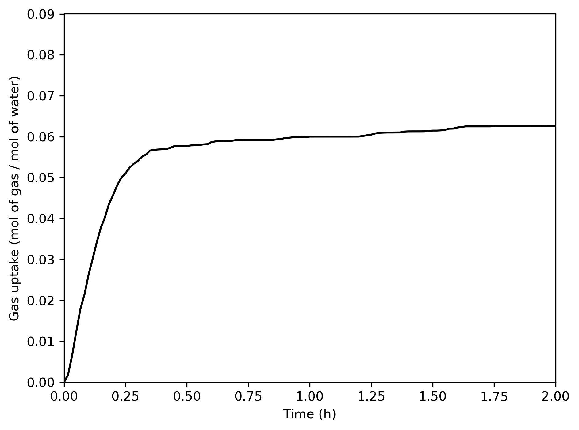
(n) Default style 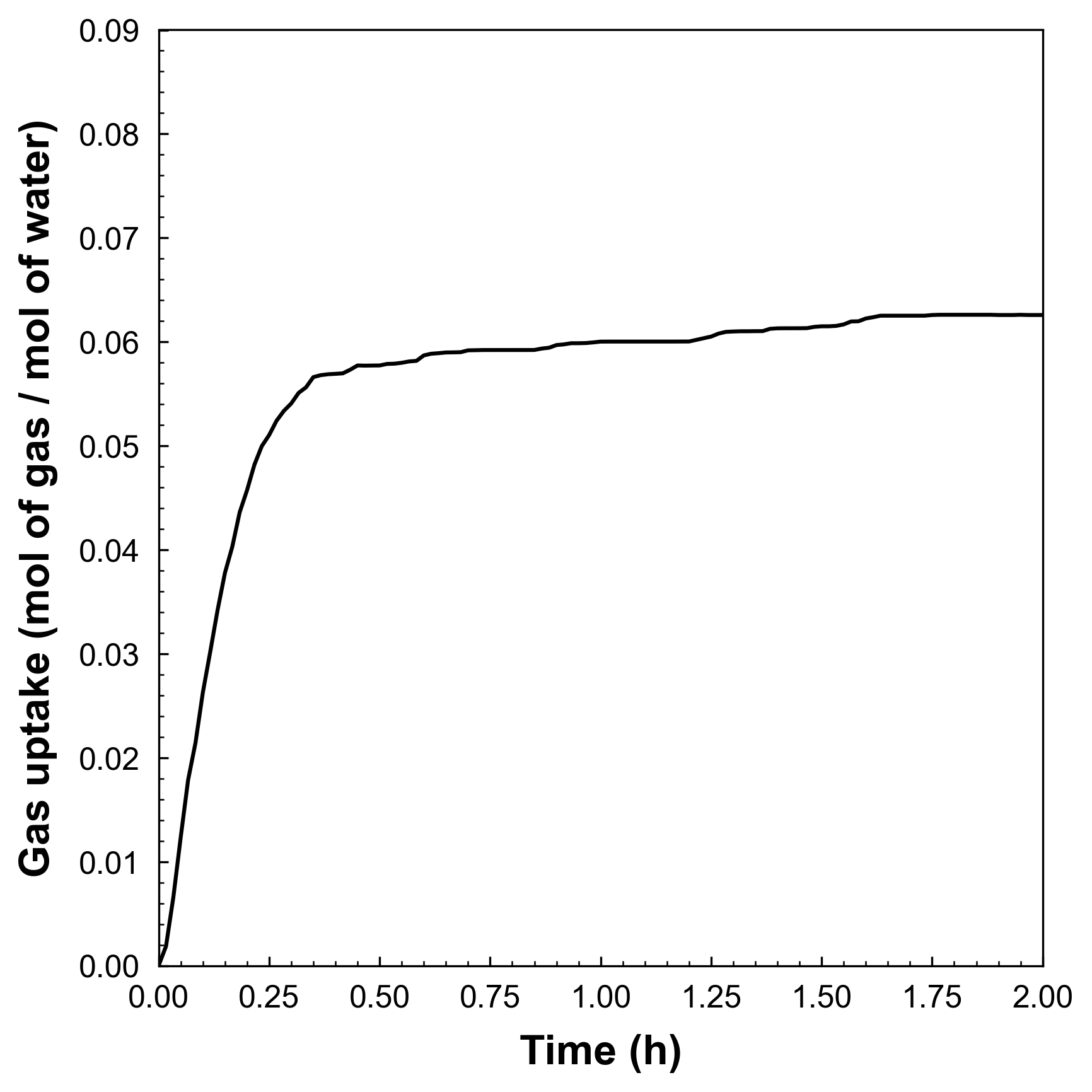
(y) Decorated style - You can also choose the equation of state model you want to use. Currently, the program supports two EOS models: Redlich-Kwong (RK) and Peng-Robinson (PR). The detailed information about the EOS models is given in the below section.
- The plot type can be either
lineorscatter.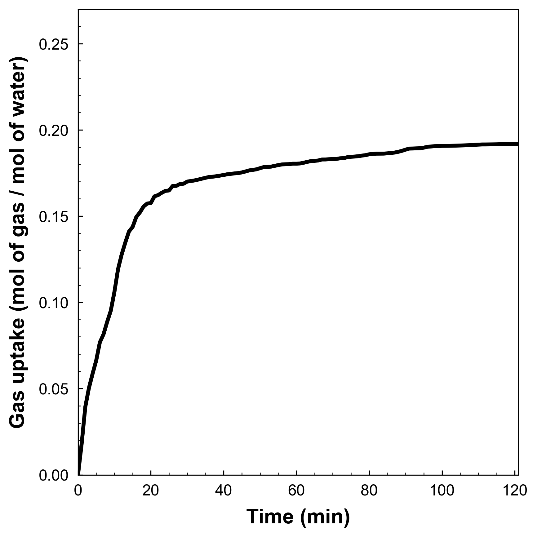
(line) Line plot 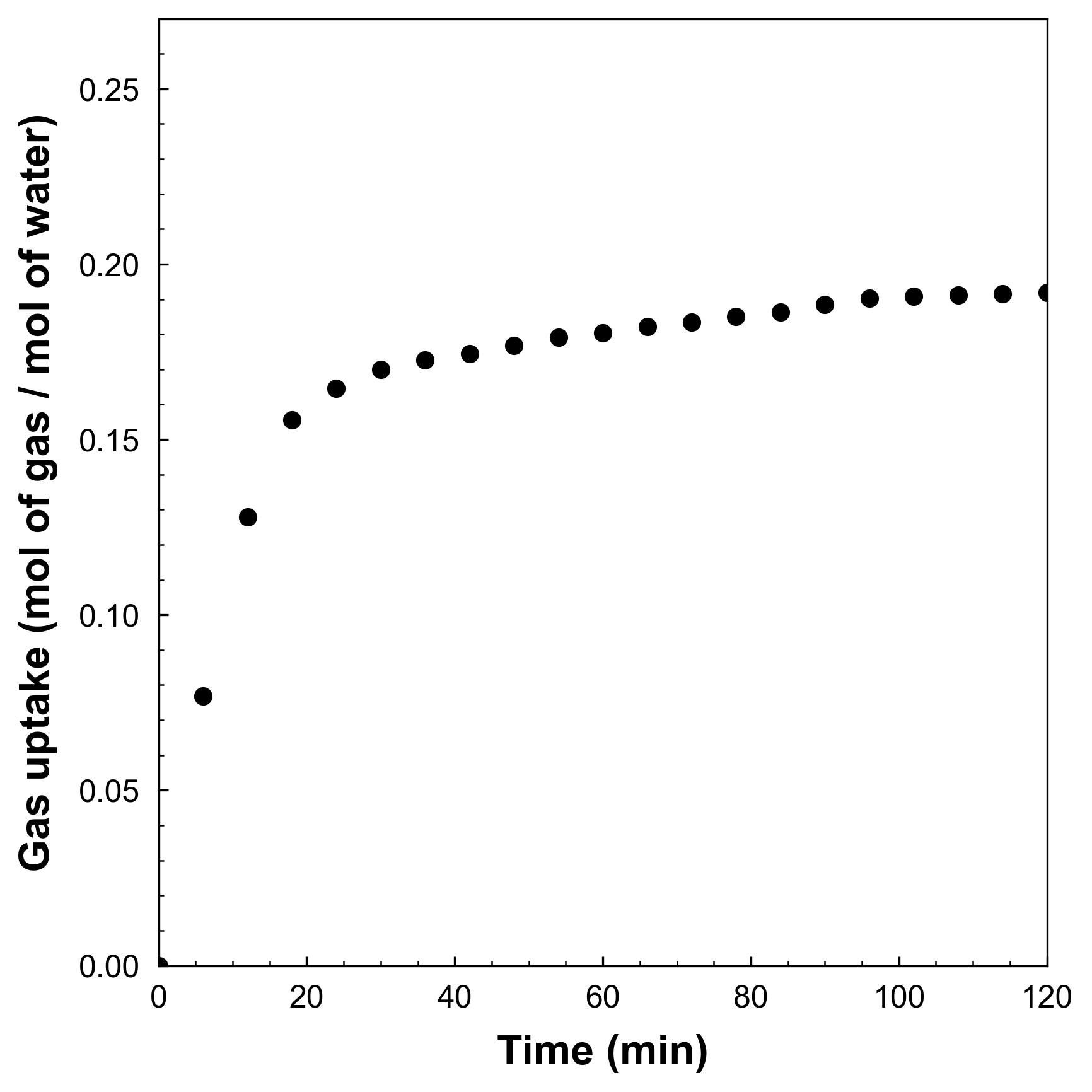
(scatter) Scatter plot - If you choose
line, the program will plot the gas uptake data with a line. Consecutively, the program will ask the line width that you want to use. - If you choose
scatter, the program will plot the gas uptake data with a scatter plot. Consecutively, the program will ask the total number of points that you want to include in the plot. The program will divide the total number of points by the number of data points you have, and then plot the data points with the same interval.
(2) Making a new output CSV
After the program outputs the graph, it collects the processed data and creates a new CSV file to provide to the user. After the program runs, check the target directory again. The file looks like this:
| Pressure (psi) | Cylinder volume (mL) | Pressure (bar) | Cylinder volume (L) | Time (min) | Delta_V (L) | Gas uptake (mol of gas) | Gas uptake (mol of gas / mol of water) |
|---|---|---|---|---|---|---|---|
| ... | ... | ... | ... | ... | ... | ... | ... |
Equation of State (EOS) information
Redlich-Kwong (RK) EOS
Redlich-Kwong EOS is one of the most popular EOSs. To calculate the compressibility factor () the program uses the following equations:
Where is the experimental temperature, is the critical temperature, is the experimental pressure, is the critical pressure, is the gas constant, and is the acentric factor. and are the parameters of the EOS.
The value is calculated by using the Newton's method.
Peng-Robinson (PR) EOS
Peng-Robinson EOS is more newer than Redlich-Kwong EOS and also one of the most popular EOSs. To calculate the compressibility factor (), the program uses the following equations:
Where is the experimental temperature, is the critical temperature, is the experimental pressure, is the critical pressure, is the gas constant, and is the acentric factor. , , and are the parameters of the Peng-Robinson EOS.
A huge thanks for @CorySimon making the Peng-Robinson Equation of State solver. It was helpful to make a function for Peng-Robinson EOS.
Equation used
Gas uptake equation
The gas uptake (mol of gas / mol of water) is simply calculated by using the following equation:
Where is the moles of gas molecules, presents the moles of water molecules, is the experimental pressure, is the volume change in ISCO syringe pump, is the compressibility factor, is the gas constant, is the experimental temperature, is the mass of water, and is the molar mass of water.
When the user select the clathrate-typeoption as sI, sII, sH, SCS-I, TS-I, and HS-I, the program will calculate the theoretical maximum gas uptake value. The program uses the following equation to calculate the theoretical maximum gas uptake value:
Where stands for the small cage, stands for the medium cage, and stands for the large cage. For semi-clathrates, stands for the pentagon-dodecahedron cage, stands for the pentadecahedron cage, and stands for the tetradecahedron cage.
If you don't want to mark the theoretical maximum gas uptake value in your plot, you can simply select the clathrate-type option as none.
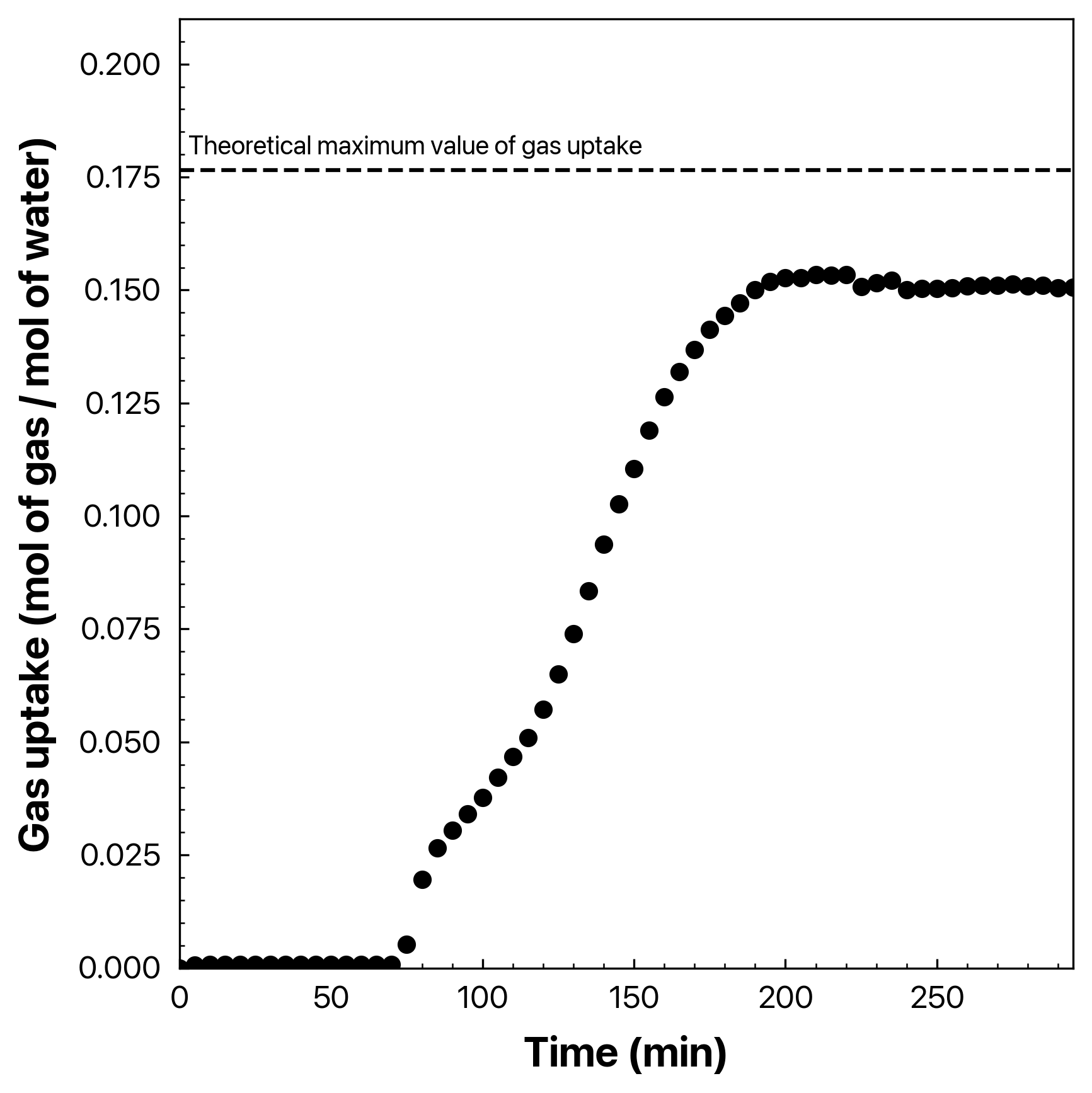
clathrate-type is on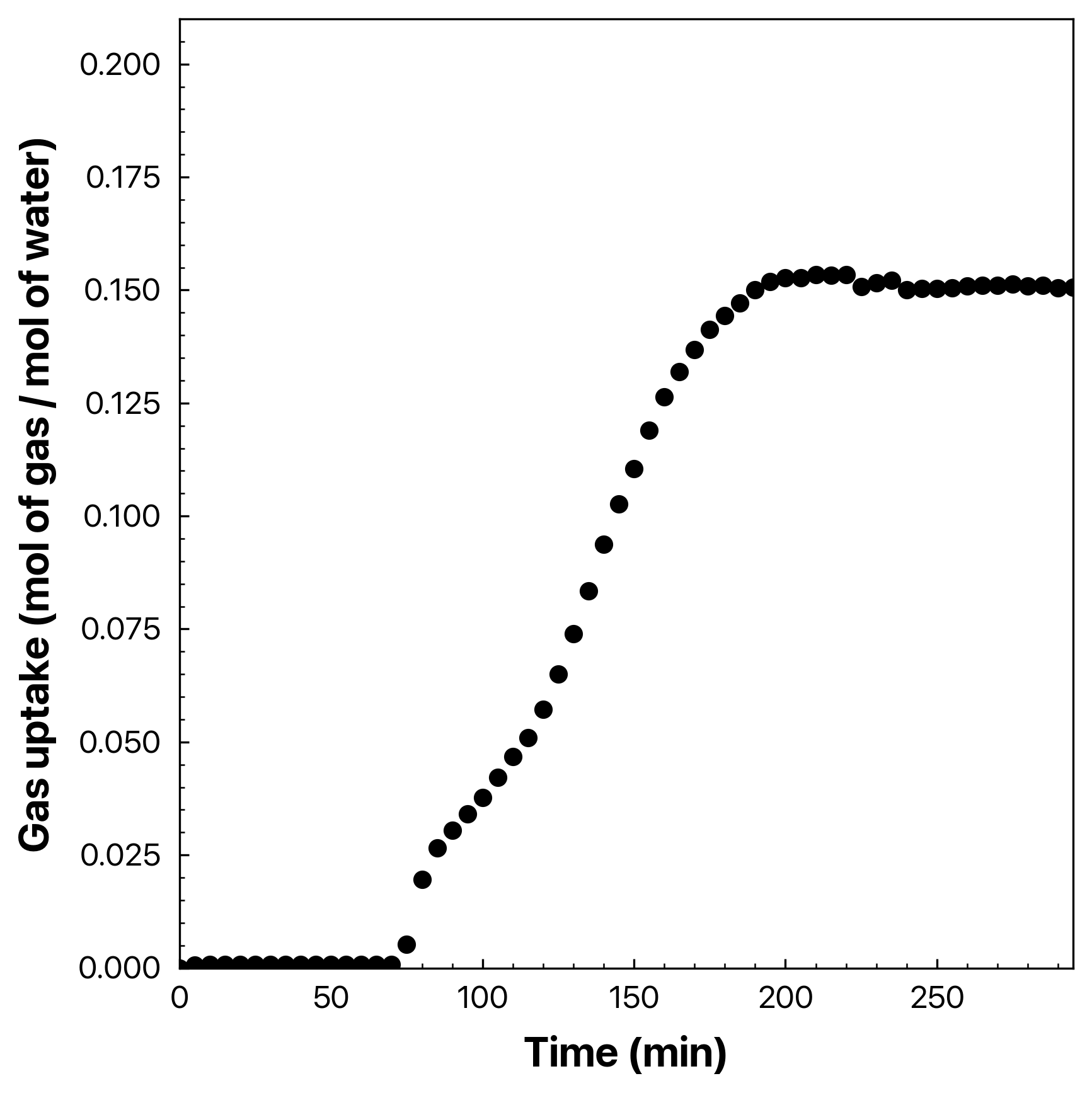
clathrate-type is noneFor advanced users
By utilizing the bash script, you can automate the sequence to treat several .csv files in your target folder. But make sure to check if it is okay to use the same settings.txt to treat your raw CSV files.
Let's see the example.
.
├── Raw1.csv
├── Raw2.csv
├── Raw3.csv
├── Raw4.csv
└── settings.txt
I put 4 raw csv files in the same directory with the pre-written settings.txt file. It looks like this:
###################################
############ SETTINGS.TXT #############
###################################
# NOTE: This file should be located in the directory where you are executing the program. This can be done by typing `pwd` in the terminal. Check your current location.
# NOTE: You can mark `#` in front of the lines you don't want to use.
# NOTE: This file should be named as `settings.txt`. If isn't, the program cannot load the settings.

###########################################################
# Target directory where the raw data files are located.
directory = ./

# Data collection frequency (in ms); the value when you set in the LabVIEW program.
frequency = 300000

# Experimental temperature (in K)
temperature = 276.3

# Critical temperature of your interested gas (in K)
tc = 209.5389

# Critical pressure of your interested gas (in bar)
pc = 55.034

# Acentric factor of your interested gas
omega = 0

# Time unit (h, m, or s)
tunit = m

# Whether to decorate the graph with research figure style (options: y, n)
graph-decorate = y

# Plot type (options: line, scatter)
plot-type = scatter

# Whether to include the title in the graph (options: y, n)
include-title = n

# Output file type (options: png, pdf, svg)
output-file-type = png

# Equation of state model (options: rk, pr)
eos = pr

# Water mass you used in the experiment (in g)
water-mass = 50

# Type of the clathrate (options: sI, sII, sH, SCS-I, TS–I, HS-I, and none)
clathrate-type = sII
Note that the gas type used in those raw files is . I wrote every , , values for , and I chose EOS as Peng-Robinson. Kr hydrate is known as sII structure, therefore, I wrote clathrate-type as sII. For the scatter plot, I chose to contain 50 points of data in every plot. The automation code looks like this:
#!/bin/bash
# advanced.sh
for filenum in 0 2 4 6
do
  autogasuptake << EOF
  $filenum
  50
EOF
done
Unfortunately, autogasuptake cannot distinguish output CSV data exported from running it. Thus, we might use the even number while the sequence loops. Authorize advanced.sh.
chmod +x advanced.shThen, execute it!
./advanced.shThen, the overall files inside the current directory might be like this:
.
├── Raw1.csv
├── Raw1.png
├── Raw1_OUTDATA.csv
├── Raw2.csv
├── Raw2.png
├── Raw2_OUTDATA.csv
├── Raw3.csv
├── Raw3.png
├── Raw3_OUTDATA.csv
├── Raw4.csv
├── Raw4.png
├── Raw4_OUTDATA.csv
├── advanced.sh
└── settings.txt
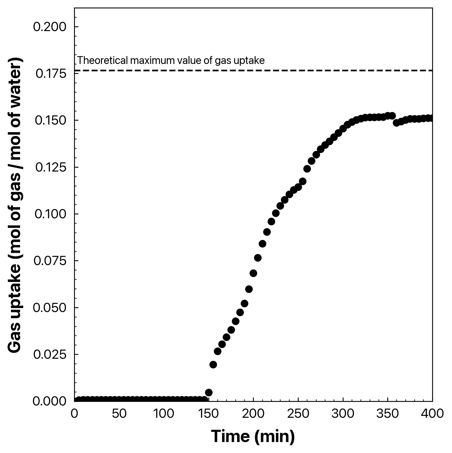
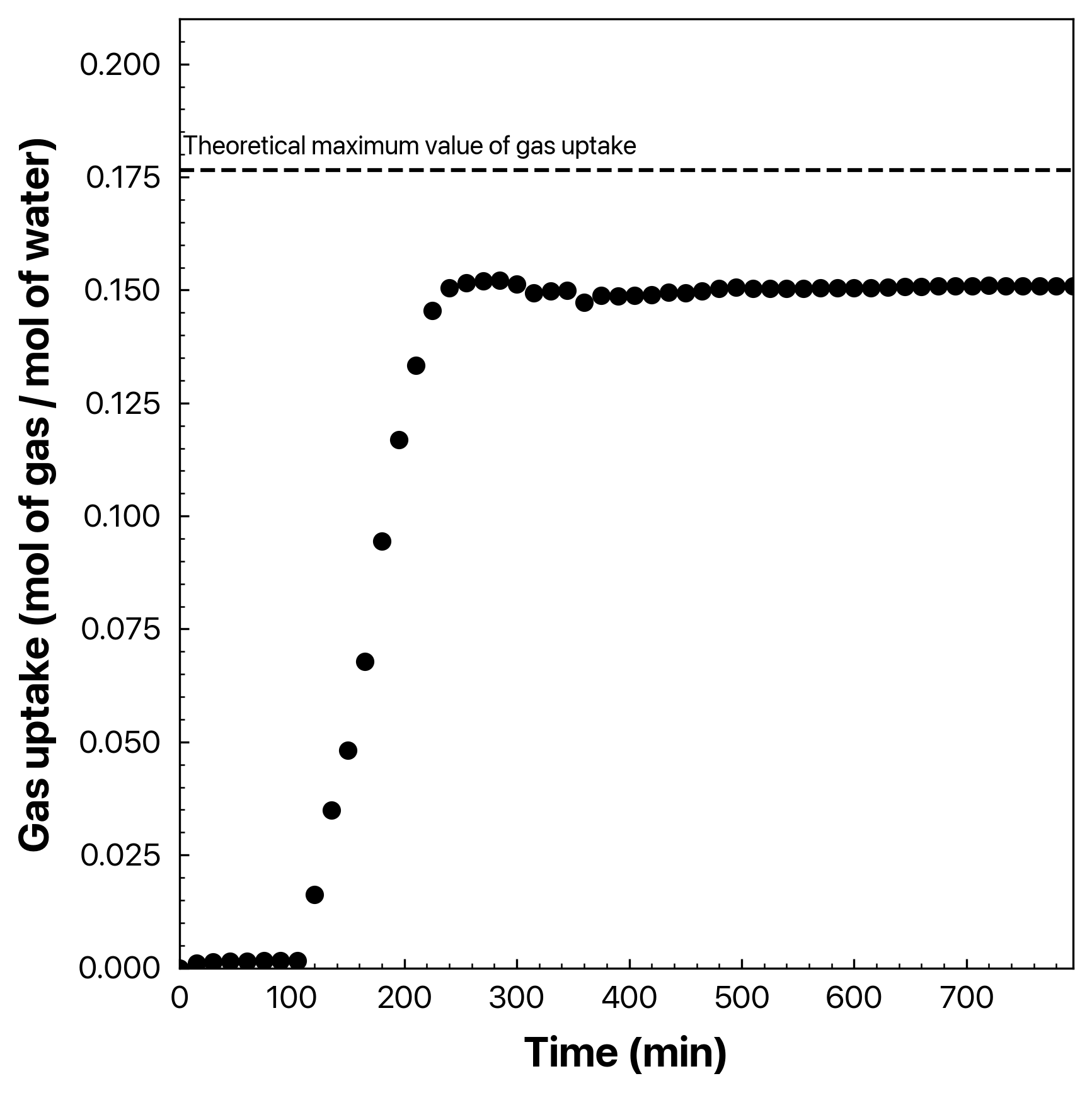
The output looks like this:
Outputs
Raw 1
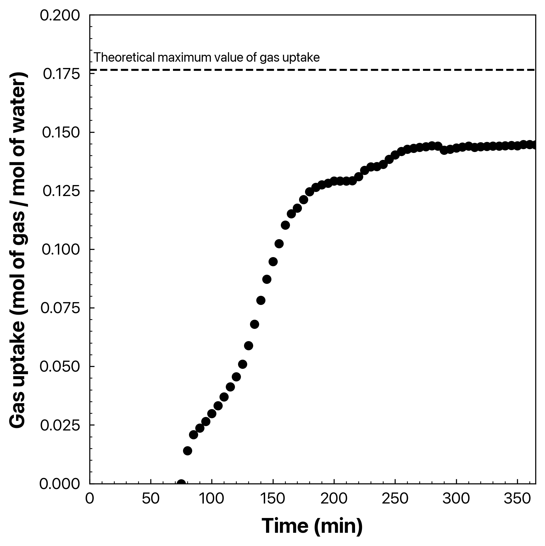
Raw 2
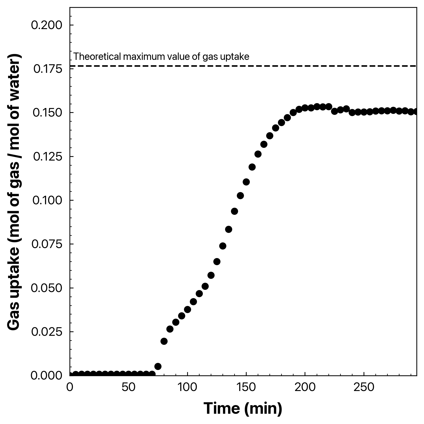
Raw 3
Raw 4
License
- MIT License